Abstract
Self-attention in Transformers comes with a high computational cost because of their quadratic computational complexity, but their effectiveness in addressing problems in language and vision has sparked extensive research aimed at enhancing their efficiency. However, diverse experimental conditions, spanning multiple input domains, prevent a fair comparison based solely on reported results, posing challenges for model selection. To address this gap in comparability, we perform a large-scale benchmark of more than 45 models for image classification, evaluating key efficiency aspects, including accuracy, speed, and memory usage. Our benchmark provides a standardized baseline for efficiency-oriented transformers. We analyze the results based on the Pareto front – the boundary of optimal models. Surprisingly, despite claims of other models being more efficient, ViT remains Pareto optimal across multiple metrics. We observe that hybrid attention-CNN models exhibit remarkable inference memory- and parameter-efficiency. Moreover, our benchmark shows that using a larger model in general is more efficient than using higher resolution images. Thanks to our holistic evaluation, we provide a centralized resource for practitioners and researchers, facilitating informed decisions when selecting or developing efficient transformers.
Introduction
The Transformer architecture [7] is one of the most successful models in deep learning, outperforming traditional models in multiple domains from language modeling to computer vision. However, a major challenge in working with Transformer models is their computational complexity of $\mathcal O(N^2)$ in the size of the input $N$. Therefore, researchers have proposed a multitude of modifications to overcome this hurdle and make Transformers more efficient.
However, it is unclear which modifications and overall strategies are the most efficient. That’s why in this paper, we will answer the following questions for the domain of image classification:
- Which specific modifications and overall strategies are the most efficient?
- Are these modifications even worth considering over the baseline transformer?
- What other dimensions influence efficiency, and how can I scale up my setup efficiently?
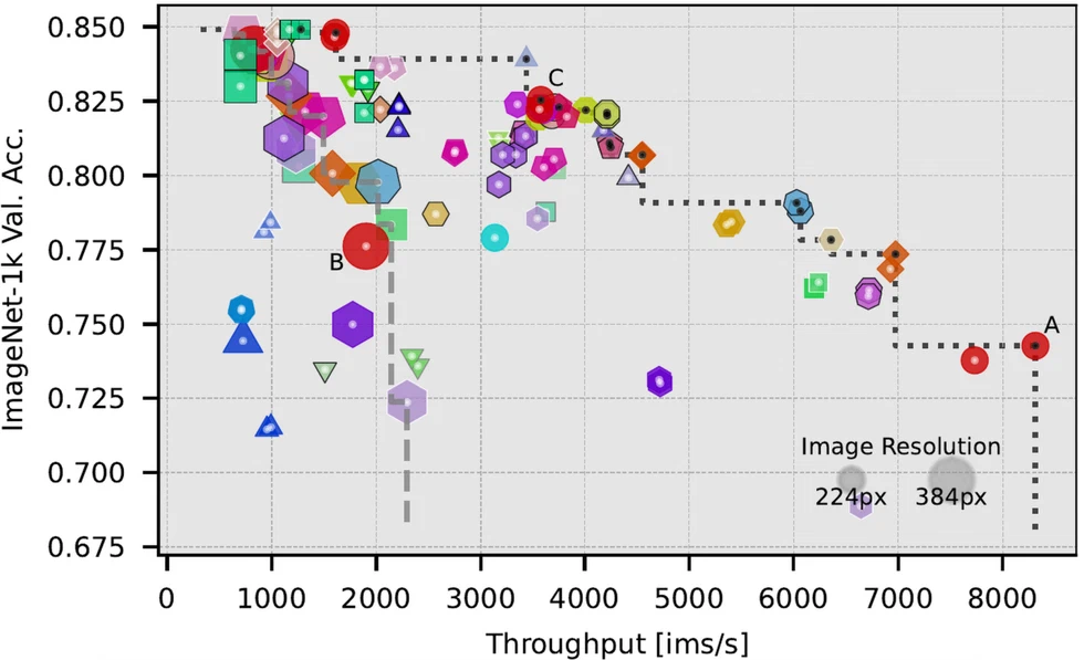
We tackle these questions by training more than 45 transformer variants from scratch, ensuring fair and comparable evaluation conditions. These transformer variants have been proposed to increase the efficiency for the domains of language or computer vision. Then we measure their speed and memory requirements, both at training and inference time. We additionally compare to the theoretical metrics of parameters and FLOPs. Our analysis is based on the Pareto front, the set of models that provide an optimal tradeoff between model performance and one aspect of efficiency. It lets us analyze the complex multidimensional tradeoffs involved in judging efficiency. In out plots, Pareto optimal models have a black dot, while the others have a white dot. For an example, see here.
To see the interactive plots, go down to the results section.
Efficient Transformers for Computer Vision
Basics of the Transformer Architecture
We briefly describe the key elements of ViT [4] (the Transformer baseline for image classification), that have been studied to make it more efficient, as well as its key bottleneck: the $\mathcal O(N^2)$ computational complexity of self-attention.
ViT is an adaption of the original Transformer, taking an image as an input, which is converted into a sequence of non-overlapping patches of size $p \times p$ (usually $p = 16$).
Each patch is linearly embedded into a token of size $d$, with a positional encoding being added.
A classification token [CLS] is appended to the sequence, which is then fed through a Transformer encoder.
There, the self-attention mechanism computes the attention weights $A$ from the queries $Q \in \mathbb R^{N \times d}$ and keys $K \in \mathbb R^{N \times d}$ for each token from the sequence:
This matrix encodes the global interactions between every possible pair of tokens, but it’s also the reason for the inherent $\mathcal O(N^2)$ computational complexity of the attention mechanism.
The output of attention is a sum over the values $V$ weighted by the attention weights: $X_\text{out} = AV$.
After self-attention, the sequence elements are passed through a 2-layer MLP.
In the end, only the [CLS] token is used for the classification decision.
Efficiency-Improving Changes
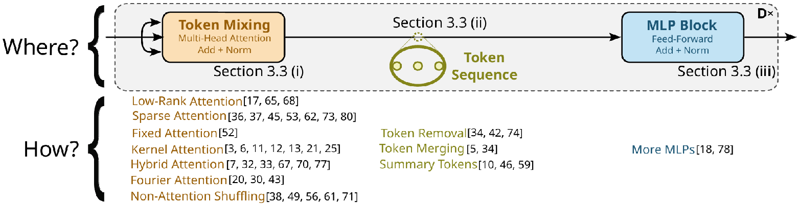
We systematically classify the efficient models using a two step approach:
- Where does the model change the baseline ViT: Ath the token-mixing mechanism, the token sequence, or at the MLP block?
- How and using what strategy does the model change the baseline?
(i) Token Mixing
The first and most popular approach is to change the token mixing mechanism, which directly tackles the $\mathcal O(N^2)$ computational complexity of self-attention. We identify 7 strategies for changing the token mixing mechanism to make it more efficient:
- Low-Rank Attention leverages the fact that $QK^\top \in \mathbb R^{N \times N}$ is a matrix of rank $r \leq d \ll N$ and approximates it by using a low-rank representation.
- Sparse Attention builds on most of the attention values being very small and only explicitly calculates a subset of values of $A$.
- Fixed Attention uses a fixed the attention matrix for all samples.
- Kernel Attention splits the $\text{softmax}$ into two functions to be applied to $Q$ and $K$ individually, so $A$ does not have to be calculated explicitly: $$ X_\text{out} = \phi(Q) \phi(K)^\top V. $$
- Hybrid Attention combines the attention mechanism with convolution layers.
- Fourier Attention uses the Fast Fourier Transform (FFT) to calculate the interactions in Fourier space with $\mathcal O(N \log N)$ complexity.
- Non-Attention Shuffling refers to other techniques of capturing interactions without using attention.
(ii) Token Sequence
Models that change up the token sequence are more prevalent in CV compared to NLP. The idea is to remove redundant information and in doing so, using the $\mathcal O(N^2)$ complexity to our advantage. Removing 30% of the tokens reduces the computational cost of self-attention by approximately 50%. The strategies we identify are:
- Token Removal: Removing unimportant tokens without losing critical information.
- Token Merging: Merging tokens to remove redundant information.
- Summary Tokens: Condensing the information from the sequence into a small set of new tokens.
(iii) MLP Block
The final way of changing the architecture was only taken by two methods. Their idea was to move computations from self-attention into the efficient MLP blocks. This is done by expanding the MLPs or exchanging self-attention layers for more MLPs.
List of Models
Experimental Design
We conduct a series of over 200 experiments on more than 45 models.
Training Pipeline
We compare models on even grounds by training from scratch with a standardized pipeline. This pipeline is based on DeiT III [6], an updated version of DeiT [5]. To reduce bias, our pipeline is relatively simple and only consists of elements commonly used in CV. In particular, we refrain from using knowledge distillation to prevent introducing bias from the choice of teacher model. Any orthogonal techniques, like quantization, sample selection, and others, are not included as they can be applied to every model and would manifest as a systematic offset in the results. To avoid issues from limited training data, we pre-train all models on ImageNet-21k [3].
Training Hyperparameters
| Pretrain | Finetune | |
|---|---|---|
| Dataset | ImageNet-21k | ImageNet-1k |
| Epochs | 90 | 50 |
| LR | $3 \times 10^{-3}$ | $3 \times 10^{-4}$ |
| Schedule | cosine decay | cosine decay |
| Batch Size | 2048 | 2048 |
| Warmup Schedule | linear | linear |
| Warmup Epochs | 5 | 5 |
| Weight Decay | 0.02 | 0.02 |
| Gradient Clipping | 1.0 | 1.0 |
| Label Smoothing | 0.1 | 0.1 |
| Drop Path Rate | 0.05 | 0.05 |
| Optimizer | Lamb | Lamb |
| Dropout Rate | 0.0 | 0.0 |
| Mixed Precision | ✅ | ✅ |
| Augmentation | 3-Augment | 3-Augment |
| Image Resolution | $224 \times 224$ or $192 \times 192$ | $224 \times 224$ or $384 \times 384$ |
| GPUs | 4 NVIDIA A100 | 4 or 8 NVIDIA A100 |
Efficiency Metrics
We track the following metrics for evaluating the model efficiency:
- Number of Parameters
- FLOPs
- Training time in GPU-hours at batch size 2048 for the full 50 epochs of finetuning on an A100 GPU
- Inference throughput in images per second at the optimal batch size on an A100 GPU
- Training memory over all GPUs during finetuing at batch size 2048
- Inference memory on a single GPU at batch size 1; the minimum amount of memory needed for inference
For comparability, the empirical metrics are measured using the same setup.
Results
Improved Training Pipeline
To validate the fairness of our training pipeline, we validate our ImageNet-1k accuracy with the original papers’ (whenever reported).
| Model | Orig. DeiT | Orig. Acc. | Our Acc. | Model | Orig. DeiT | Orig. Acc. | Our Acc. | |
|---|---|---|---|---|---|---|---|---|
| ViT-S (DeiT) | ✅ | 79.8 | 82.54 | ViT-S (DeiT III) | 82.6 | 82.54 | ||
| XCiT-S | ✅ | 82.0 | 83.65 | Swin-S | ✅ | 83.0 | 84.87 | |
| Swin-V2-Ti | 81.7 | 83.09 | Wave-ViT-S | 82.7 | 83.61 | |||
| Poly-SA-ViT-S | 71.48 | 78.34 | SLAB-S | ✅ | 80.0 | 78.70 | ||
| EfficientFormer-V2-S0 | 75.7${}^D$ | 71.53 | CvT-13 | 83.3$\uparrow$ | 82.35 | |||
| CoaT-Ti | ✅ | 78.37 | 78.42 | EfficientViT-B2 | 82.7$\uparrow$ | 81.53 | ||
| NextViT-S | 82.5 | 83.92 | ResT-S | ✅ | 79.6 | 79.92 | ||
| FocalNet-S | 83.4 | 84.91 | SwiftFormer-S | 78.5${}^D$ | 76.41 | |||
| FastViT-S12 | ✅ | 79.8$\uparrow$ | 78.77 | EfficientMod-S | ✅ | 81.0 | 80.21 | |
| GFNet-S | 80.0 | 81.33 | EViT-S | ✅ | 79.4 | 82.29 | ||
| DynamicViT-S | 83.0${}^D$ | 81.09 | EViT Fuse | ✅ | 79.5 | 81.96 | ||
| ToMe-ViT-S | ✅ | 79.42 | 82.11 | TokenLearner-ViT-8 | 77.87$\downarrow$ | 80.66 | ||
| STViT-Swin-Ti | ✅ | 80.8 | 82.22 | CaiT-S24 | ✅ | 82.7 | 84.91 |
We find that 13 out of 26 papers base their training pipelines on DeiT, making our pipeline a good fit. Additionally, we see that with our pipeline accuracy increases by $0.85$% on average. Most models reporting higher performance using the original pipeline were trained with knowledge distillation (which we avoid to reduce bias) or using a larger image resolution (which we show is inefficient).
Number of Parameters
Use widescreen format for the best view of the interactive plots.
We find that in general, the accuracy per parameter goes down as models get larger. This is especially the case with the ViT models, which are more parameter efficient than similar accuracy models at smaller sizes (ViT-Ti) and less parameter efficient for the larger models (ViT-B). The most parameter efficient models are Hybrid Attention models (EfficientFormerV2-S0, CoaT-Ti) and other Non-attention shuffling models which incorporate convolutions (SwiftFormer, FastViT).
Speed
Inference Throughput
The models we evaluate often claim a superior throughput vs. accuracy trade-off compared to ViT. However, we find that ViT remains Pareto optimal at all model sizes. Only few models (Synthesizer-FR, NextViT, and some Token Sequence models) show improvements in the Pareto front when compared to a ViT of comparable size. We find that these observations replicate on other datasets and even when using CPUs instead of GPUs.
Training Speed
This Pareto front is very similar to the one for inference time. Here, some Token Sequence models are highly efficient; in particular TokenLearner.
Generally, ViT is still a solid choice for speed.
Memory
Training Memory
Training memory again exhibits a similar pattern as above. There is a stark contrast between models using low-resolution and high-resolution images as the ones with high-resolution images need significantly more memory with not that much accuracy gained.
Inference Memory
The Pareto front of inference memory is the most different to all the others. It is the only one where ViT is not Pareto optimal. Instead Hybrid Attention and convolution based models excel, similar to the number of parameters. It is also the only setup where a model (EviT) using 384px resolution images is Pareto optimal.
Scaling Behaviors
Our observations reveal that fine-tuning at a higher resolution is inefficient. While it may result in improved accuracy, it entails a significant increase in computational cost, leading to a substantial reduction in throughput. In turn, scaling up the model ends up being more efficient. This can be seen when comparing the corresponding Pareto fronts for throughput, training speed, and training memory.
A few examples for scaling the model vs. scaling the image size:
We see that scaling up the model size is always more efficient than scaling up the image resolution.Correlation of Metrics
| $\text{corr}(x, y)$ | Params | Training Time | Training Memory | Inference Time | Inference Memory |
|---|---|---|---|---|---|
| FLOPS | 0.30 | 0.72 | 0.85 | 0.48 | 0.42 |
| Params | 0.05 | 0.18 | 0.02 | 0.40 | |
| Training Time | 0.89 | 0.81 | 0.17 | ||
| Training Memory | 0.71 | 0.48 | |||
| Inference Time | 0.13 |
The highest correlation of 0.89 is between fine-tuning time and training memory. This suggests a common underlying factor or bottleneck, possibly related to the necessity of memory reads during training. We find a reliability of estimating computational costs only based on theoretical metrics, like [1, 2] before. Consequently, assessing model efficiency in practice requires the empirical measurement of throughput and memory requirements.
TlDr: Which Transformer to Favor?
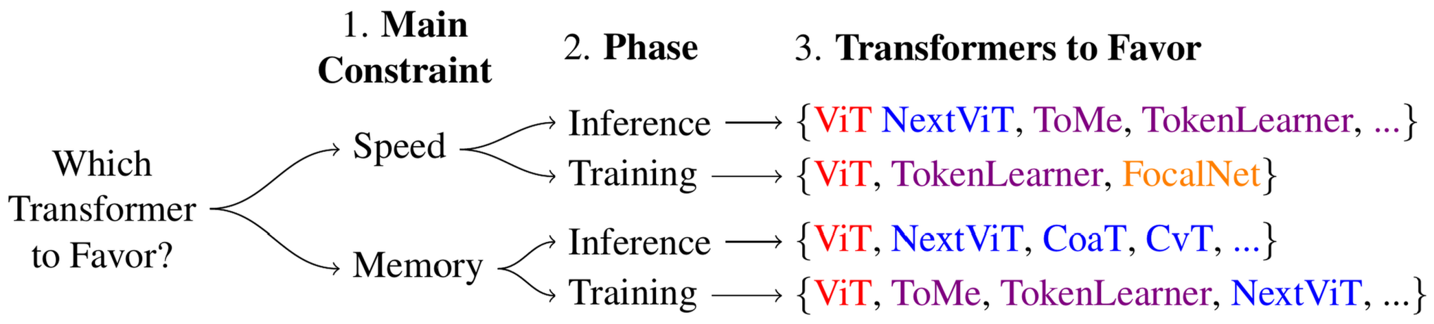
Our benchmark offers actionable insights for answering the question of which transformer to favor in the form of models and strategies to use. We have compiled an overview of these in the flowchart above. ViT remains the preferred choice overall. However, Token Sequence methods can become viable alternatives when speed and training efficiency are of importance. For scenarios with significant inference memory constraints, considering Hybrid CNN-attention models can prove advantageous.
We additionally find that it is much more efficient to scale up the model size than to scale up the image resolution. This goes against the trend of efficient models being evaluated using higher resolution images, which cancels out possible efficiency gains.
References
For references and links to the efficient transformer models, see the list of models.
- Brian R Bartoldson, Bhavya Kailkhura, and Davis Blalock. Compute-efficient deep learning: Algorithmic trends and opportunities. Journal of Machine Learning Research, 24(122):1–77, 2023.
- Mostafa Dehghani, Yi Tay, Anurag Arnab, Lucas Beyer, and Ashish Vaswani. The efficiency misnomer. In International Conference on Learning Representations, 2022.
- Jia Deng, Wei Dong, Richard Socher, Li-Jia Li, Kai Li, and Li Fei-Fei. ImageNet: A large-scale hierarchical image database. In 2009 IEEE Conference on Computer Vision and Pattern Recognition. IEEE, 2009.
- Alexey Dosovitskiy, Lucas Beyer, Alexander Kolesnikov, Dirk Weissenborn, Xiaohua Zhai, Thomas Unterthiner, Mostafa Dehghani, Matthias Minderer, Georg Heigold, Sylvain Gelly, Jakob Uszkoreit, and Neil Houlsby. An image is worth 16x16 words: Transformers for image recognition at scale. In 9th International Conference on Learning Rep- resentations, ICLR 2021, Virtual Event, Austria, May 3-7, 2021. OpenReview.net, 2021.
- Hugo Touvron, Matthieu Cord, Matthijs Douze, Francisco Massa, Alexandre Sablayrolles, and Herve Jegou. Training data-efficient image transformers & distillation through attention. In Marina Meila and Tong Zhang, editors, Proceedings of the 38th International Conference on Machine Learning, volume 139 of Proceedings of Machine Learning Research, pages 10347–10357. PMLR, 7 2021.
- Hugo Touvron, Matthieu Cord, and Hervé Jégou. Deit iii: Revenge of the vit. In Shai Avidan, Gabriel Brostow, Moustapha Cissé, Giovanni Maria Farinella, and Tal Hassner, editors, Computer Vision – ECCV 2022, pages 516–533, Cham, 2022. Springer Nature Switzerland.
- Ashish Vaswani, Noam Shazeer, Niki Parmar, Jakob Uszkoreit, Llion Jones, Aidan N Gomez, Lukasz Kaiser, and Illia Polosukhin. Attention is all you need. In I. Guyon, U. Von Luxburg, S. Bengio, H. Wallach, R. Fergus, S. Vishwanathan, and R. Garnett, editors, Advances in Neural Information Processing Systems, volume 30. Curran Associates, Inc., 2017.
Citation
If you use this work, please cite our paper:
@inproceedings{Nauen2024WTFBenchmark,
  author = {Nauen, Tobias Christian and Palacio, Sebastian and Raue, Federico
            and Dengel, Andreas},
  title = {Which Transformer to Favor: A Comparative Analysis of Efficiency in
           Vision Transformers},
  booktitle = {Proceedings of the Winter Conference on Applications of Computer
               Vision (WACV)},
  month = {February},
  year = {2025},
  pages = {6955-6966},
}