Abstract
The quadratic complexity of the attention mechanism represents one of the biggest hurdles for processing long sequences using Transformers. Current methods, relying on sparse representations or stateful recurrence, sacrifice token-to-token interactions, which ultimately leads to compromises in performance. This paper introduces TaylorShift, a novel reformulation of the Taylor softmax that enables computing full token-to-token interactions in linear time and space. We analytically determine the crossover points where employing TaylorShift becomes more efficient than traditional attention, aligning closely with empirical measurements. Specifically, our findings demonstrate that TaylorShift enhances memory efficiency for sequences as short as 800 tokens and accelerates inference for inputs of approximately 1700 tokens and beyond. For shorter sequences, TaylorShift scales comparably with the vanilla attention. Furthermore, a classification benchmark across five tasks involving long sequences reveals no degradation in accuracy when employing Transformers equipped with TaylorShift. For reproducibility, we provide access to our code on GitHub.
Introduction
Despite their remarkable success, Transformers face a significant challenge when dealing with long sequences due to the quadratic complexity of the attention mechanism. This limitation hinders their application to tasks involving extensive contextual information, such as processing long documents or high-resolution images. While various approaches have been proposed to address this issue, they often sacrifice accuracy, specialize in specific domains, or neglect individual token-to-token interactions. To overcome these limitations, we introduce TaylorShift, a novel method that reformulates the softmax function in the attention mechanism using the Taylor approximation of the exponential. By combining this approximation with a tensor-product-based operator, TaylorShift achieves linear-time complexity while preserving the essential token-to-token interactions. We analyze the efficiency of TaylorShift in depth, both analytically and empirically and find that it outperforms the standard transformer architecture in 4 out of 5 tasks.
How does TaylorShift work?
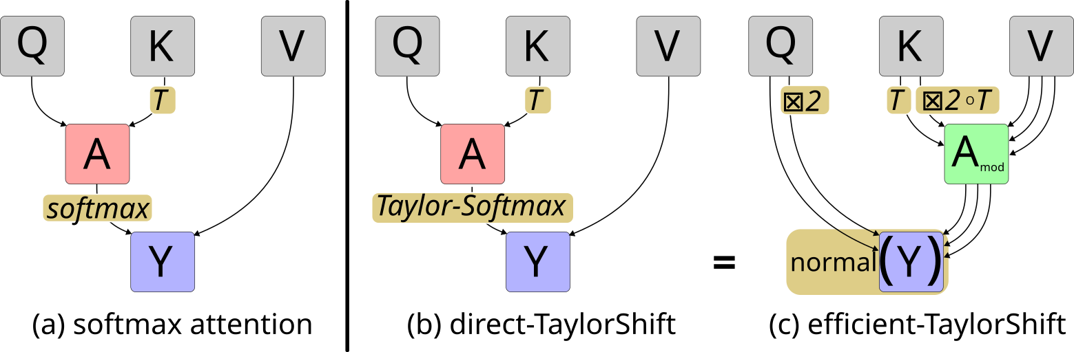
Essentially, TaylorShift works by replacing the exponential function in the softmax by its Taylor approximation. For a vector $\mathbf x = [x\_1, ..., x\_m] = [x_i]_{i = 1}^m$:
$$ \text{softmax}(x) = \left[\frac{\exp(x_i)}{\sum\_{j} \exp(x_j)}\right]\_{i = 1}^m \approx \left[ \frac{\frac{x_i^2}{2} + x_i + 1}{\sum_j \frac{x_j^2}{2} + x_j + 1} \right]\_{i = 1}^m = \text{T-SM}(x) $$Direct TaylorShift
We call the direct implementation of the attention mechanism using the Taylor Softmax direct-TaylorShift, as seen here. For queries $Q$, keys $K$, and values $V$, this becomes:
$$ Y = \text{T-SM}(Q K^\top) V $$Efficient TaylorShift
Direct-TaylorShift has the same scaling behavior as standard attention. However, we can reduce its computational complexity from $\mathcal O(N^2 d)$ to $\mathcal O(N d^3)$ by reordering the operations internally. This becomes useful for long sequences, where $N \gg d$.
Let me first introduce a tensor-product-based operator:
$$ \boxtimes: \mathbb R^{N \times d} \times \mathbb R^{N \times d} \to \mathbb R^{N \times d^2}. $$Basically, we take two lists of $d$-dimensional vectors $[a\_i \in \mathbb R^d]\_i$ and $[b\_i \in \mathbb R^i]\_i$ and for each index $i$ we multiply each element of $a_i$ with all the elements of $b_i$. The result is $d^2$ dimensional, since that is the number of possible combinations. We also write $A^{\boxtimes 2} := A \boxtimes A$.
Mathematical Details
In mathematical terms, we define $$ [A \boxtimes B]_n = \iota(A_n \otimes B_n) \in \mathbb R^{d^2} \hspace{10pt} \forall n=1, ..., N $$ Here, $A_n$, $B_n$, and $[A \boxtimes B]_n$ is the $n$-th entry of the respective matrix. $\otimes$ is the tensor product (or outer product) of two $d$-dimensional vectors and $\iota: \mathbb R^{d \times d} \to \mathbb R^{d^2}$ is the canonical isomorphism (basically, it just reorders the entries of a matrix into a vector; the exact order does not matter, as long as it's always the same one).It turns out, that by using this operator, we can calculate TaylorShift more efficiently:
$$ Y = Y_\text{nom} \oslash Y_\text{denom} = \left[ \frac{[Y_\text{nom}]\_{i, :}}{[Y_\text{denom}]\_i} \right]\_{i = 1}^N $$with
$$ Y_\text{nom} = \frac 1 2 Q^{\boxtimes 2} \left( (K^{\boxtimes 2})^\top V \right) + Q (K^\top V) + \sum_\text{columns} V. $$$Y_\text{denom}$ is the same, but with $\mathbb 1 = [1, ..., 1]$ instead of $V$.
Mathematical Details
We have $$ Y_\text{nom} = \frac 1 2 (Q K^\top)^{\odot 2} V + Q K^\top V + \sum_\text{columns} V. $$ Let $ \pi: \{1, .., d\} \times \{1, ..., d\} \to \{1, ..., d^2\} $ be the map that describes the reordering that $\iota$ (defined in the Mathematical Details section above) does. Then we have $$ \left[ A^{\boxtimes 2} \right]_{n, \pi(k, \ell)} = (A_n \otimes A_n)_{k, \ell} = A_{n, k} A_{n, \ell}. $$ This allows us to linearize the squared term $(Q K^\top)^{\odot 2} V$ by using $\boxtimes$ to unroll the square of a sum along a sum of $d^2$ elements: $$ \begin{align*} \left[(QK^\top)^{\odot 2} \right]_{i, j} =& \left( \sum_{k = 1}^d Q_{ik} K_{jk} \right)^2 \\ =& \sum_{k, \ell = 1}^d Q_{ik} Q_{i\ell} K_{jk} K_{j \ell} \\ =& \sum_{k, \ell = 1}^d \left[ Q^{\boxtimes 2} \right]_{i, \pi(k, \ell)} \left[ K^{\boxtimes 2} \right]_{j, \pi(k, \ell)} \\ =& \left[ Q^{\boxtimes 2} \right]_i \left[ K^{\boxtimes 2} \right]_j^\top \end{align*} $$ Therefore $$ (QK\top)^{\odot 2} V = Q^{\boxtimes 2} (K^{\boxtimes 2})^\top V, $$ which can be computed in $\mathcal O(N d^3)$ by multiplying from right to left. We can also calculate $Y_\text{nom}$ and $Y_\text{denom}$ at once by setting $V \gets V \circ \mathbb 1$.Normalization
We found that some intermediate results of TaylorShift tended to have very large norms, which ultimately led to training failures. We introduce the following three steps for normalization:
- Normalize the queries and keys to one and introduce an additional attention temperature parameter (per attention-head) $\tau \in \mathbb R$: $$ q_i \gets \frac{\tau q_i}{||q_i||_2}, \hspace{10pt} k_i \gets \frac{k_i}{||k_i||_2} \hspace{10pt} \forall i=1, ..., N $$
- Counteract the scaling behaviors by multiplying $Q$ and $K$ by $\sqrt[4]{d}$ and $V$ by $\frac 1 N$.
- Normalize the output by multiplying by $\sqrt{\frac N d}$.
Scaling Behavior Details
Experimentally, we find the following approximate mean sizes for intermediate results with $Q, K,$ and $V$ sampled uniformly from the unit sphere:| Interm. Expr. | $(K^{\boxtimes 2})^\top V$ | $(QK^\top)^{\odot 2} V$ | $ QK^\top V$ | $Y_\text{denom}$ | $Y$ |
|---|---|---|---|---|---|
| Size ($\approx$) | $\frac{N}{\sqrt d}$ | $\frac N d$ | $\sqrt N (1 + \frac{1}{4d})$ | $N (2 + \frac{1}{d})$ | $\sqrt{\frac d N}$ |
| Size after Normalization ($\approx$) | $1$ | $1$ | $\frac{1}{\sqrt{Nd}} (1 + \frac{1}{4d})$ | $2 + \frac{1}{d}$ | $1$ |
Efficient-TaylorShift Algorithm
We compile all the information into the pseudocode for efficient-TaylorShift:
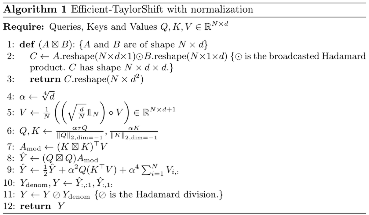
Find the PyTorch implementation here.
How efficient is efficient-TaylorShift?
We analyze the circumstances where efficient-TaylorShift is more efficient than direct-TaylorShift in terms of speed, based on the number of floating point operations, and memory, based on the size of intermediate results.
Floating Point Operations
The number of floating point operations for direct-TaylorShift and efficient-TaylorShift is
$$\text{ops}_\text{dir} = 4N^2 d + 6 N^2,$$$$\text{ops}\_\text{eff} = N (4d^3 + 10d^2 + 9d + 4).$$Therefore, there exists an $N_0 = N_0(d)$, such that efficient-TaylorShift is more efficient for all $N > N_0$. We calculate
$$ N_0 = \frac{4d^3 + 10d^2 + 9d + 4}{4d + 6} \leq d^2 + d + \frac 3 4. $$Mathematical Details
We need the following operations:direct-TaylorShift:
- $2N^2 d$ for the multiplication of $QK^\top$,
- $4N^2$ operations to apply $x \mapsto \frac 1 2 x^2 + x + 1$ element-wise to that matrix,
- $2N^2$ operations for normalization,
- $2N^2 d$ operations for the final multiplication by $V$ $$ \Rightarrow \text{ops}_\text{dir} = 4 N^2 d + 6 N^2 $$
efficient-TaylorShift:
- $2N d^2$ operations for $K^{\boxtimes 2}$ and $Q^{\boxtimes 2}$,
- $2 N d^2 (d + 1)$ operations to multiply by $V \in \mathbb R^{N \times (d+1)}$ and get $(K^{\boxtimes 2})^\top V$,
- $2 N d^2 (d + 1)$ operations for the final multiplication by $Q^{\boxtimes 2}$,
- $4 N d (d + 1)$ operations for computing $Q K^\top V$ from right to left,
- $N (d + 1)$ operations for summing up the columns of $V$,
- $3 N (d + 1)$ operations for the sums and scalar multiplication, and finally
- $N d$ operations for normalization. $$ \Rightarrow \text{ops}_\text{eff} = N (2 d^2 + 4 d^2 (d + 1) + 4 d (d + 1) + 4 (d + 1) + d) $$
We derive $N_0$ by setting $\text{ops}\_\text{dir} \stackrel{!}{=} \text{ops}\_\text{eff}$, which is equivalent to
$$ N_0 = \frac{4d^3 + 10d^2 + 9d + 4}{4d + 6} \leq \frac{4d^3 + 6d^2}{4d + 6} + \frac{4d^2 + 6d}{4d + 6} + \frac{3d + 4.5}{4d + 6} = d^2 + d + \frac 3 4 $$Size of intermediate Results
The size of the largest intermediate results needed at once for direct- and efficient-TaylorShift is
$$\text{entries}_\text{dir} = \underbrace{dN}\_{\text{for } V} + \underbrace{2N^2}\_{\text{for } QK^\top \text{ and result}},$$$$\text{entries}\_\text{eff} = d^2(d+1) + 2dN + (d+1)N + d^2N.$$We can again find $N_1 = N_1(d)$, such that efficient-TaylorShift is more memory efficient for all $N > N_1$. We find
$$ N_1 = \frac 1 4 \left[ d^2 + 2 d + 1 + \sqrt{d^4 + 12 d^3 + 14 d^2 + 4d + 1} \right] \leq \frac 1 2 d^2 + 2 d + \frac 1 2. $$Mathematical Details
We count the number of entries in the largest intermediate results needed at once.For direct-TaylorShift we need the largest intermediate memory when calculating $\text{T-SM}(QK^\top)$ from $QK^\top$.
- $d N$ entries of $V$
- $N^2$ entries of $QK^\top$
- $N^2$ entries for the result. Note that we can’t simply reuse the memory from $QK^\top$, because we need to save at least one intermediate result when calculating $\frac 1 2 x^2 + x$.
For efficient-TaylorShift we need the most memory when calculating $(K^{\boxtimes 2})^\top V$:
- $2 N d$ entries for $Q,$ and $K$ for later
- $N (d + 1)$ entries for $V$ (also needed again later)
- $N d^2$ entries of $K^{\boxtimes 2}$
- $d^2 (d + 1)$ entries for the result
We again derive $N_1$ by setting $\text{entries}\_\text{dir} \stackrel{!}{=} \text{entries}\_\text{eff}$ for $N_1$. Therefore
$$ N_1^2 - \frac{d^2 + 2d + 1}{2} N_1 - \frac{d^3 + d^2}{2} = 0 $$The larger of the two solutions is
$$ \begin{align*} N_1 =& \frac 1 4 \left[ d^2 + 2d + 1 + \sqrt{(d^2 + 2d + 1)^2 + 8(d^3 + d^2)} \right] \\\\ =& \frac 1 4 \left[ d^2 + 2d + 1 + \sqrt{d^4 + 12 d^3 + 14 d^2 + 4d + 1} \right]. \end{align*} $$Since
$$ (d^2 + 6d + 1)^2 = d^4 + 12d^3 + 38 d^2 + 12 d + 1 \geq d^4 + 12 d^3 + 14 d^2 + 4d + 1 $$we have
$$ N_1 \leq \frac 1 2 d^2 + 2 d + \frac 1 2. $$$N_0$ and $N_1$ for typical values of $d$
Table:
| d | 8 | 16 | 32 | 64 | 128 |
|---|---|---|---|---|---|
| $N_0$ | 73 | 273 | 1057 | 4161 | 16513 |
| $N_1$ | 47 | 159 | 574 | 2174 | 8446 |
Calculator:
d =
=> N_0 = 1057 N_1 = 577
How can we increase the efficiency?
In an effort to increase the efficiency while processing the same number of tokens $N$, one might opt to reduce the embedding dimension $d_\text{emb}$. However, this might come at the cost of expressiveness. Given that efficient-TaylorShift scales with $\mathcal O(Nd^3)$, we can instead increase the number of attention heads $h$ with dimension $d = \frac{d_\text{emb}}{h}$ each. We find that the number of operations is
$$ \text{ops}\_\text{eff}(\text{MHSA}) = N \left( 4 \frac{d\_\text{emb}^3}{h^2} + 10 \frac{d\_\text{emb}^2}{h} + 9 d\_\text{emb} + 4h \right) $$and the number of entries is
$$ \text{entries}\_\text{eff}(\text{MHSA}) = \frac{d\_\text{emb}^3}{h^2} + (N + 1) \frac{d\_\text{emb}^2}{h} + 3N d\_\text{emb} + N h, $$which are both strictly decreasing in $h$. Therefore, efficient-TaylorShift becomes faster and needs less memory with more attention heads.
Mathematical Details
We identify the extreme points of both (as functions of $h$) by setting their derivatives to zero: $$ \frac{\partial}{\partial h} \text{ops}_\text{eff}(\text{MHSA}) = -8 \frac{d_\text{emb}^3}{h^3} - 10 \frac{d_\text{emb}^2}{h^2} + 4 $$ By setting $d = \frac{d_\text{emb}}{h}$, we find that the above is zero at $d \approx 0.52$. This would imply $h = \frac{1}{0.52} d_\text{emb}$, but the maximum value for $h$ is $d_\text{emb}$, since the number of dimensions $d$ has to be an integer.Similarly, for the number of entries, we find:
$$ \frac{\partial}{\partial h} \text{entries}\_\text{eff}(\text{MHSA}) = -2 d^2 - (N + 1) d + N \stackrel{!}{=} 0 $$$$ \Leftrightarrow N = (2d + N + 1) d^2 \stackrel{d > 0}{\geq} (N + 1) d^2 $$Therefore $1 > \frac{N}{N+1} \geq d^2$ which would imply $1 > d$ and therefore $h > d_\text{emb}$ again, but the maximum value possible is $h = d_\text{emb}$.
Empirical Evaluation
Efficiency of TaylorShift Attention
We first validate our theoretical analysis on the efficiency of TaylorShift by measuring its inference time and memory usage under different configurations of $d$ and $N$:
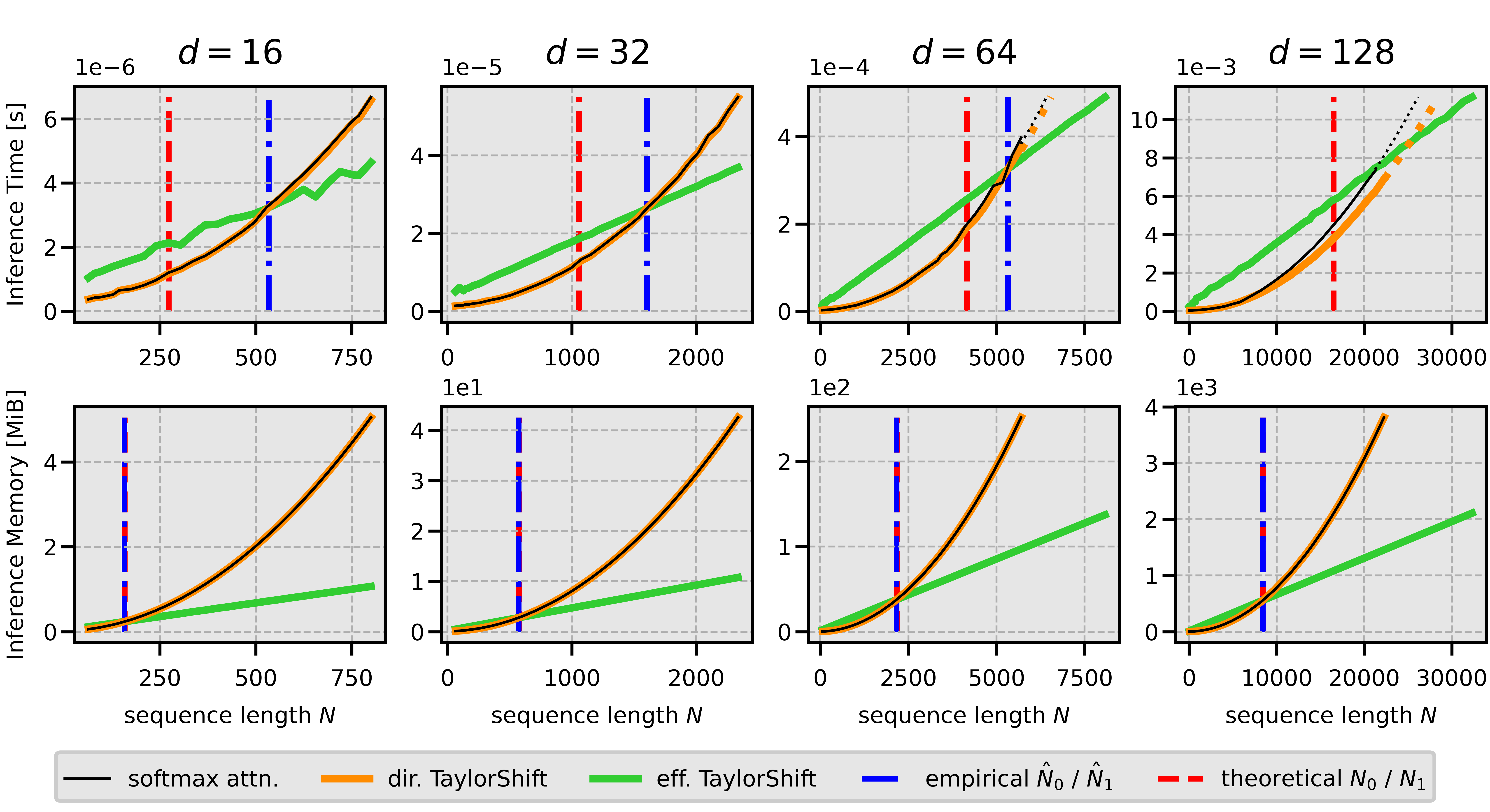 We observe that the empirical estimate for the memory transition point $\hat N_1$ coincides almost exactly with the theoretical value $N_1$, with an error of at most $0.6\%$.
The difference between the empirical speed transition point $\hat N_0$ and the theoretical one $N_0$ is approximately proportional to $d$: $\hat N_0 - N_0 \approx 18 d$.
We hypothesize that the more sequential nature of efficient-TaylorShift results in more, costly reads and writes in GPU memory.
It might indicate possible efficiency gains for efficient-TaylorShift from a low-level IO-efficient implementation.
We observe that the empirical estimate for the memory transition point $\hat N_1$ coincides almost exactly with the theoretical value $N_1$, with an error of at most $0.6\%$.
The difference between the empirical speed transition point $\hat N_0$ and the theoretical one $N_0$ is approximately proportional to $d$: $\hat N_0 - N_0 \approx 18 d$.
We hypothesize that the more sequential nature of efficient-TaylorShift results in more, costly reads and writes in GPU memory.
It might indicate possible efficiency gains for efficient-TaylorShift from a low-level IO-efficient implementation.
Performance of a Transformer with TaylorShift
We test the accuracy of multiple (efficient) Transformers on a set of 5 tasks from the Long Range Arena benchmark [4], as well as ImageNet classification at two model sizes. We use the same standard hyperparameters for all models. Models with * had to be trained in full instead of mixed precision. All tasks are classitication tasks and the table shows accuracy in percent.
| Model | CIFAR (Pixel) | IMDB (Byte) | ListOps | ImageNet (Ti) | ImageNet (S) | Average |
|---|---|---|---|---|---|---|
| Linformer [6] | 29.2 | 58.1 | – | 64.3 | 76.3 | (57.0) |
| RFA [3] | 44.9 | 65.8 | – | – | – | (55.4) |
| Performer [1] | 34.2* | 65.6* | 35.4* | 62.0* | 67.1* | 52.9 |
| Reformer [2] | 44.8 | 63.9 | 47.6 | 73.6 | 76.2* | 61.2 |
| Nyströmformer [7] | 49.4 | 65.6 | 44.5 | 75.0 | 78.3* | 62.6 |
| EVA [8] | 46.1 | 64.0 | 45.3 | 73.4 | 78.2 | 61.4 |
| Transformer [5] | 44.7 | 65.8 | 46.0 | 75.6 | 79.1 | 62.2 |
| TaylorShift (ours) | 47.6 | 66.2 | 46.1 | 75.0 | 79.3 | 62.8 |
This shows TaylorShift’s consistent performance across various datasets. It surpasses all other models on 4 out of 5 datasets, positioning itself as a good all-rounder model. We observe a notable increase of $4.3\%$ when transitioning from size Ti to S on ImageNet, in contrast to $3.5\%$ for the Transformer, which highlights TaylorShifts scalability.
Number of attention heads
We train TaylorShift models on the pixel-level CIFAR10 task to see how accuracy and efficiency change. All models have the default $d_\text{emb} = 256$ with $d = \frac{d_\text{emb}}{h}$ in the attention mechanism. The default is $h = 4$.
| $h$ | $d$ | Acc [%] | dir-TS TP [ims/s] | dir-TS Mem [MiB@16] | eff-TS TP [ims/s] | eff-TS Mem [MiB@16] |
|---|---|---|---|---|---|---|
| 4 | 64 | 47.1 | 12060 | 596 | 2975 | 840 |
| 8 | 32 | 47.5 | 7657 | 1111 | 5749 | 585 |
| 16 | 16 | 47.3 | 4341 | 2135 | 9713 | 459 |
| 32 | 8 | 46.9 | 2528 | 4187 | 14087 | 397 |
| 64 | 4 | 45.9 | 1235 | 8291 | 13480 | 125 |
We see that increasing the number of attention heads $h$ increases the speed and decreases the memory needed by efficient-TaylorShift, as predicted. Additionally, we find that it also increases the performance up to a certain point. Until there, we have a win-win-win situation with a faster, more lightweight and more accurate model. After that the number of heads can be used to trade off accuracy against the amount compute needed.
Conclusion & Outlook
We introduced TaylorShift a novel efficient Transformer model. It offers significant computational advantages without sacrificing performance. By approximating the exponential function, TaylorShift achieves linear time and memory complexity, making it ideal for long sequences. Our experiments demonstrate its superiority over standard Transformers in terms of speed, memory efficiency, and even accuracy.
As we move forward, we envision TaylorShift opening up new possibilities for tackling challenging tasks involving lengthy sequences. From high-resolution image processing to large-scale document analysis, TaylorShift’s efficiency and versatility make it a promising tool for the future of efficient Transformer models.
References
- K.M. Choromanski, V. Likhosherstov, D. Dohan, X. Song, A. Gane, T. Sarlos, P. Hawkins, J.Q. Davis, A. Mohiuddin, L. Kaiser, D.B. Belanger, L.J. Colwell, and A. Weller “Rethinking attention with performers”. ICLR 2021.
- N. Kitaev, L. Kaiser, and A. Levskaya. “Reformer: The efficient transformer”. ICLR 2020.
- H. Peng, N. Pappas, D. Yogatama, R. Schwartz, N.A. Smith, and L. Kong “Random feature attention”. ICLR 2021.
- Y. Tay, M. Dehghani, S. Abnar, Y. Shen, D. Bahri, P. Pham, J. Rao, L. Yang, S. Ruder, and D. Metzler “Long range arena: A benchmark for efficient transformers” ICLR 2021.
- A. Vaswani, N. Shazeer, N. Parmar, J. Uszkoreit, L. Jones, A.N. Gomez, L. Kaiser, and I. Polosukhin “Attention is all you need”. NeurIPS 2017.
- S. Wang, B.Z. Li, M. Khabsa, H. Fang, and H. Ma “Linformer: Self-attention with linear complexity”. ArXiv Prerint 2020.
- Y. Xiong, Z. Zeng, R. Chakraborty, M. Tan ,G. Fung, Y. Li, and V. Singh “Nyströmformer: A nyström-based algorithm for approximating self-attention”. AAAI 2021.
- L. Zheng, J. Yuan, C. Wang, and L. Kong “Efficient attention via control variates”. ICLR 2023.
Citation
If you use this work, please cite our paper:
@inproceedings{Nauen2024TaylorShift,
  title = {TaylorShift: Shifting the Complexity of Self-Attention from Squared
           to Linear (and Back) using Taylor-Softmax},
  author = {Tobias Christian Nauen and Sebastian Palacio and Andreas Dengel},
  note = {ICPR 2024 (oral)},
  editor = {Antonacopoulos, Apostolos and Chaudhuri, Subhasis and Chellappa,
            Rama and Liu, Cheng-Lin and Bhattacharya, Saumik and Pal, Umapada},
  booktitle = {Pattern Recognition},
  year = {2024},
  publisher = {Springer Nature Switzerland},
  address = {Cham},
  pages = {1--16},
  isbn = {978-3-031-78172-8},
  doi = {10.1007/978-3-031-78172-8_1},
}